Python Interface

The zndraw package provides a Python interface to interact with the visualisation tool. To use this API, you need to have a running instance of the ZnDraw web server.

Getting Started

Start a local webserver using the command line interface:

$ zndraw file.xyz --port 1234

Then connect from Python:

from zndraw import ZnDraw

vis = ZnDraw(url="http://localhost:1234", room="123e4567-e89b-12d3-a456-426614174000/my-room")

Note

Each visualisation is associated with a room address of the form <owner_uuid>/<name> (visible in the URL). Use this address to interact via Python API or share with others. Single-segment names are no longer supported.

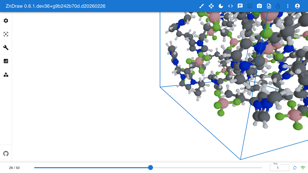
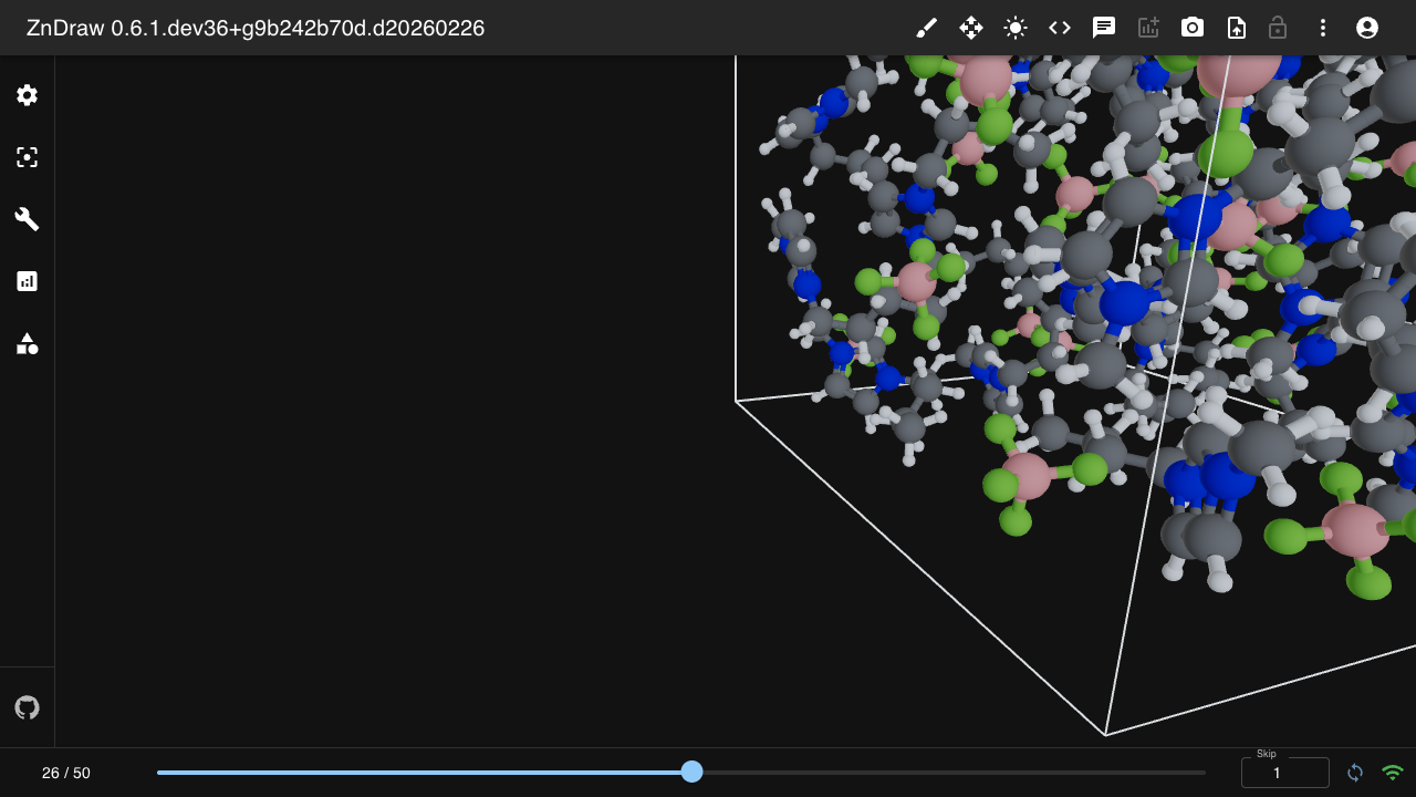
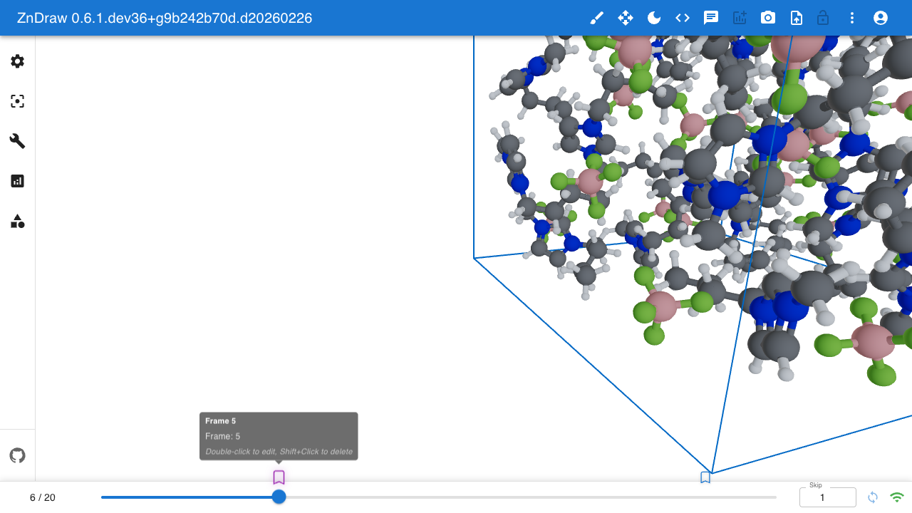
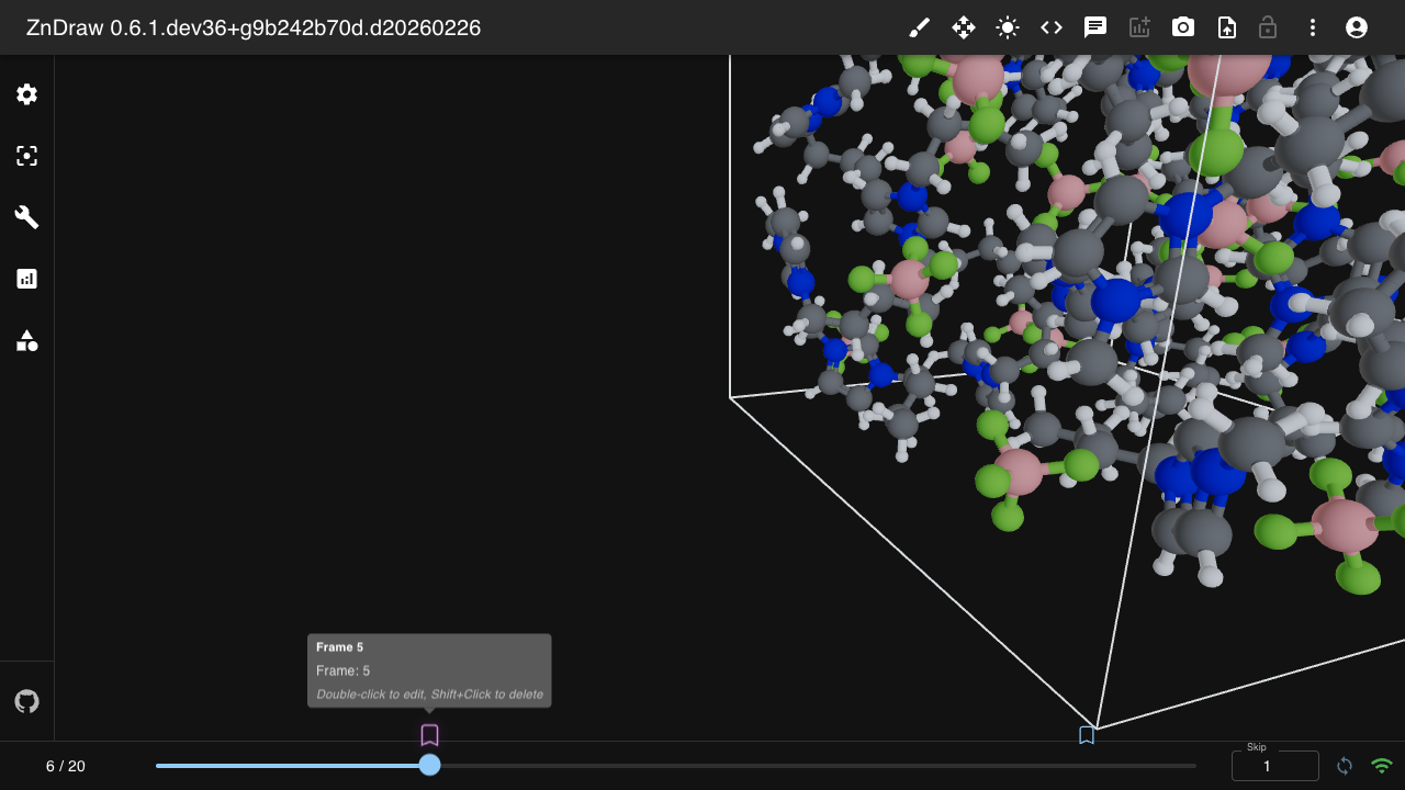
Click the connection info button in the UI to see how to connect from Python:

Authentication

ZnDraw supports optional user authentication:

vis = ZnDraw(
    url="http://localhost:1234",
    room="123e4567-e89b-12d3-a456-426614174000/my-room",
    user="my-username",
    password="my-password"
)

If no user is provided, the server will assign a guest username.

Working with Frames

The vis object behaves like a Python list of ase.Atoms objects. Modifying the list updates the visualisation in real-time.

import ase.io as aio

# Load and display frames
frames = aio.read("file.xyz", index=":")
vis.extend(frames)

# Access frames
atoms = vis[vis.step]  # Current frame
subset = vis[10:20]    # Slice of frames

# Iterate
for atoms in vis:
    print(atoms)

# Navigate to a specific frame
vis.step = 25

Selections

Select atoms by index using vis.selection (shortcut for particles geometry):

# Set selection for particles
vis.selection = [0, 1, 2, 3]

# Get selection
selected = vis.selection

# Clear selection
vis.selection = []

Select by geometry type using vis.selections (dict-like interface):

# Set selection for specific geometry
vis.selections["particles"] = [0, 1, 2, 3]
vis.selections["forces"] = [5, 6, 7]

# Get selection for a geometry
particle_selection = vis.selections["particles"]

# Clear selection for a geometry
del vis.selections["particles"]

# Iterate over geometries with selections
for geometry in vis.selections:
    print(f"{geometry}: {vis.selections[geometry]}")

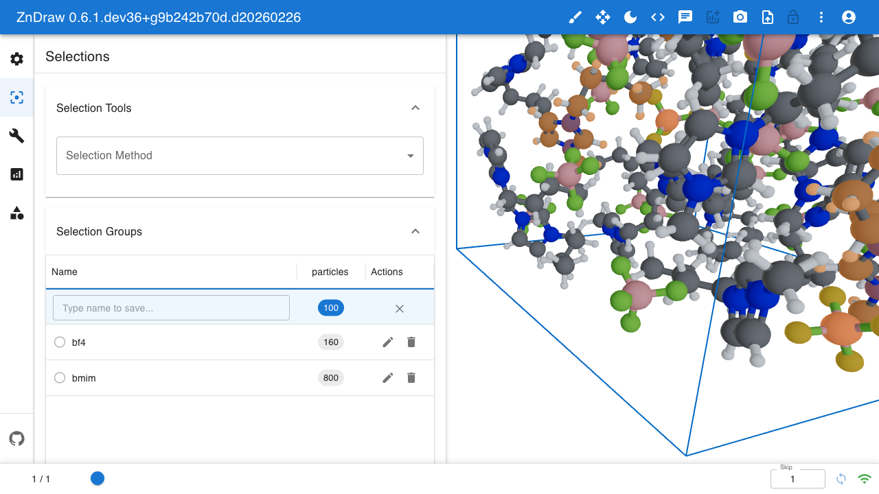
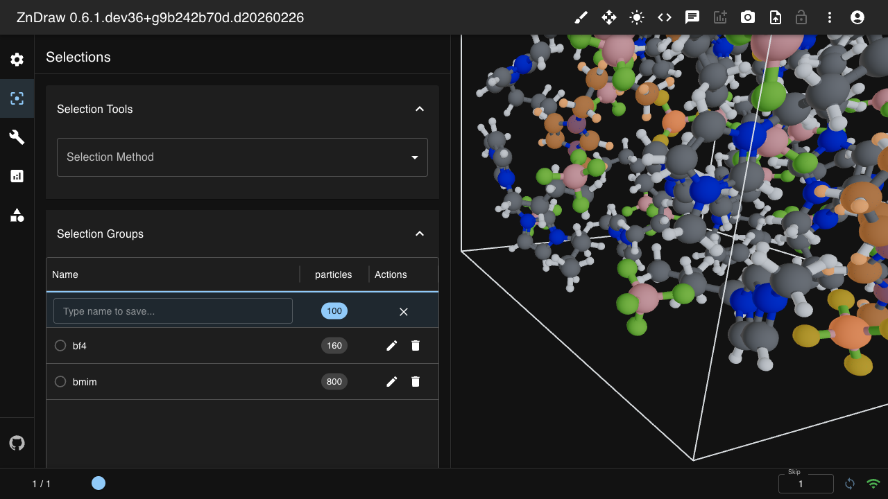
Use selection groups to save and restore named selections across multiple geometries:

# Create named group (maps geometry names to indices)
vis.selection_groups["backbone"] = {
    "particles": [0, 1, 2],
    "forces": [0, 1, 2]
}

# Create group with only particles
vis.selection_groups["active_site"] = {"particles": [10, 11, 12]}

# Get a group
group = vis.selection_groups["backbone"]
print(group)  # {"particles": [0, 1, 2], "forces": [0, 1, 2]}

# Load a group (apply it to current selections)
vis.load_selection_group("backbone")

# List all groups
for group_name in vis.selection_groups:
    print(f"{group_name}: {vis.selection_groups[group_name]}")

# Delete a group
del vis.selection_groups["backbone"]

Bookmarks

Label important frames with bookmarks:

# Add bookmark to frame 0
vis.bookmarks[0] = "Initial State"

# Add bookmark to frame 50
vis.bookmarks[50] = "Transition"

# List all bookmarks
for frame, label in vis.bookmarks.items():
    print(f"Frame {frame}: {label}")

# Delete bookmark
del vis.bookmarks[0]

Geometries

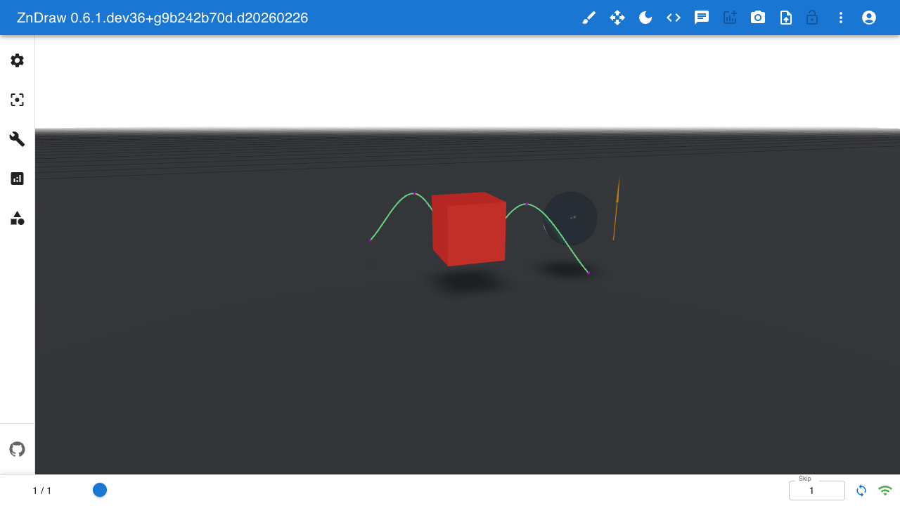
Add 3D geometries to the scene using vis.geometries:

from zndraw.geometries import Box, Sphere, Curve, Arrow, Floor

# Add a floor
vis.geometries["floor"] = Floor(active=True, position=(0, -2.0, 0), color="#808080")

# Add a red box with cartoon material
vis.geometries["box"] = Box(
    position=[(0, 2, 0)],
    size=[(4, 4, 4)],
    color=["#e74c3c"],
    material="MeshToonMaterial"
)

# Add a blue sphere with glass material
vis.geometries["sphere"] = Sphere(
    position=[(8, 2, 0)],
    radius=[2.0],
    color=["#3498db"],
    material="MeshPhysicalMaterial_glass"
)

# Add a green curve
vis.geometries["curve"] = Curve(
    position=[(-6, 0, -6), (-3, 4, -3), (0, 0, 0), (3, 4, 3), (6, 0, 6)],
    color="#2ecc71"
)

# Add an orange arrow with shiny material
vis.geometries["arrow"] = Arrow(
    position=[(12, 0, 0)],
    direction=[(0, 5, 0)],
    color=["#f39c12"],
    material="MeshPhysicalMaterial_shiny"
)

# List geometries
print(list(vis.geometries.keys()))

# Delete geometry
del vis.geometries["box"]

Available materials: MeshPhysicalMaterial_matt (default), MeshPhysicalMaterial_glass, MeshPhysicalMaterial_shiny, MeshToonMaterial, MeshStandardMaterial_metallic, and more.

Curve Customization

Curves use CatmullRom spline interpolation between control points. Customize the curve appearance with additional parameters:

from zndraw.geometries import Curve, CurveMarker

vis.geometries["curve"] = Curve(
    position=[(-6, 0, -6), (-3, 4, -3), (0, 0, 0), (3, 4, 3), (6, 0, 6)],
    color="#2ecc71",
    divisions=100,  # Interpolation smoothness (1-200, default 50)
    thickness=3.0,  # Line thickness (0.5-10, default 2.0)
    marker=CurveMarker(
        enabled=True,    # Show control point markers
        size=0.15,       # Marker size (0.01-1.0)
        color="default", # Use curve color, or specify hex
        opacity=1.0,     # Marker opacity (0-1)
    ),
    virtual_marker=CurveMarker(
        enabled=True,    # Show markers between control points
        size=0.1,        # Smaller than main markers
        opacity=0.5,     # Semi-transparent
    ),
)

Marker Settings:

• marker: Settings for control point markers (the main editable points)

• virtual_marker: Settings for markers between control points (shown in editing mode, click to insert new control point)

Both marker types support:

• enabled: Show or hide markers

• size: Marker size (0.01 to 1.0)

• color: Hex color or "default" to use curve color

• opacity: Transparency (0 = invisible, 1 = opaque)

• selecting: Appearance when selected (color, opacity)

• hovering: Appearance when hovered (color, opacity)

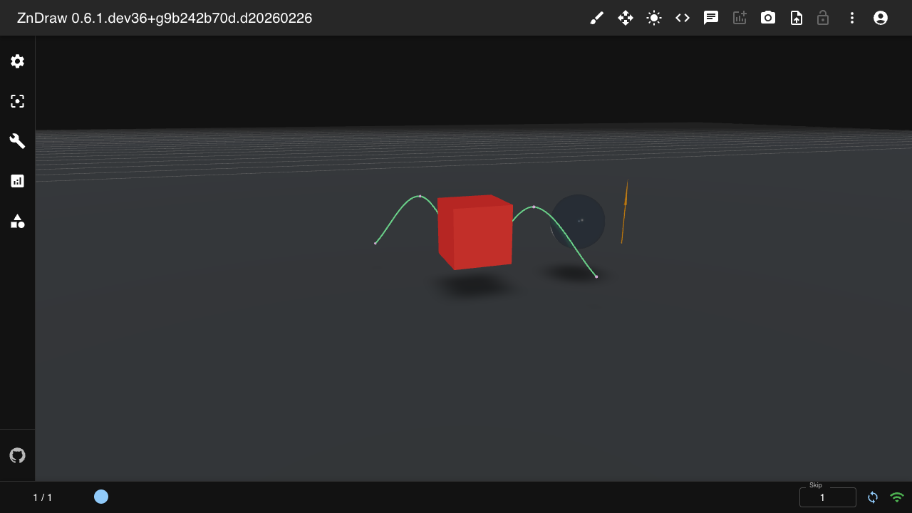
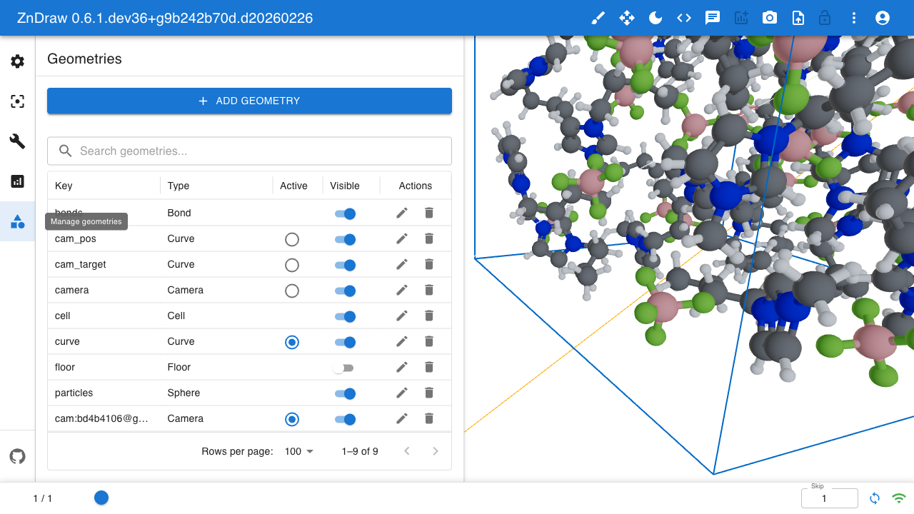
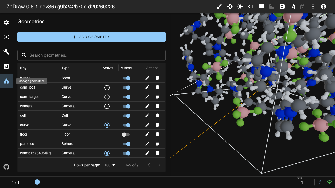
Manage geometries through the UI panel:

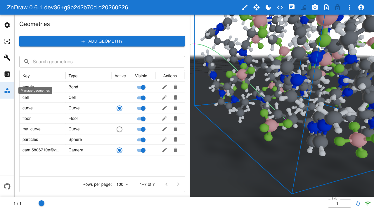
Camera Control

Control the camera programmatically. Cameras can use direct coordinates for static positions or CurveAttachment to follow curve paths for animations:

from zndraw.geometries import Camera, Curve
from zndraw.transformations import CurveAttachment

# Static camera with direct coordinates
vis.geometries["camera"] = Camera(
    position=(0, 5, 10),
    target=(0, 0, 0),
    fov=60
)

# Animated camera following curves
vis.geometries["cam_path"] = Curve(
    position=[(25, 15, 25), (30, 20, 15), (25, 15, 5)],
    color="#3498db"
)
vis.geometries["target_path"] = Curve(
    position=[(10, 10, 10), (12, 10, 10), (10, 10, 10)],
    color="#e74c3c"
)

vis.geometries["camera"] = Camera(
    position=CurveAttachment(geometry_key="cam_path", progress=0.5),
    target=CurveAttachment(geometry_key="target_path", progress=0.5),
    fov=60,
    helper_visible=True,
    helper_color="#00ff00"
)

You can mix direct coordinates with CurveAttachment:

# Camera follows curve but always looks at origin
vis.geometries["camera"] = Camera(
    position=CurveAttachment(geometry_key="flight_path", progress=0.0),
    target=(0, 0, 0),  # Fixed target
    fov=60
)

Camera parameters:

• position: Direct (x, y, z) coordinates or CurveAttachment

• target: Direct (x, y, z) coordinates or CurveAttachment

• fov: Field of view in degrees (1-179, default 50)

• camera_type: CameraType.PERSPECTIVE or CameraType.ORTHOGRAPHIC

• helper_visible: Show camera cone visualization

• helper_color: Color of the helper (hex or named)

• near, far: Clipping planes

• zoom: Camera zoom factor

Default Camera

Set a default camera so that new browser sessions start with a specific view:

from zndraw.geometries import Camera

# Create a template camera
vis.geometries["template-cam"] = Camera(
    position=(10, 10, 30),
    target=(0, 0, 0),
    fov=60
)

# Set as default for new sessions
vis.default_camera = "template-cam"

# Check current default
print(vis.default_camera)  # "template-cam"

# Unset
vis.default_camera = None

When set, new frontend sessions joining the room will clone the default camera’s position, target, fov, and other properties instead of using model defaults.

In the UI, the default camera is indicated with a star icon in the geometry grid. Click the star to toggle the default camera setting.

Drawing Mode

Draw curve control points interactively in the 3D view.

Entering Drawing Mode:

1. Press X to enter drawing mode (from view mode)

2. A drawing marker appears at your cursor position

3. Click to add control points to the active curve

4. Press X again to exit and return to view mode

The drawing marker shows where a new point will be added. It turns red when the cursor is over an invalid position.

Note

Drawing mode only works with Curve geometries that have static positions. See Keyboard Shortcuts for the complete list of keyboard controls.

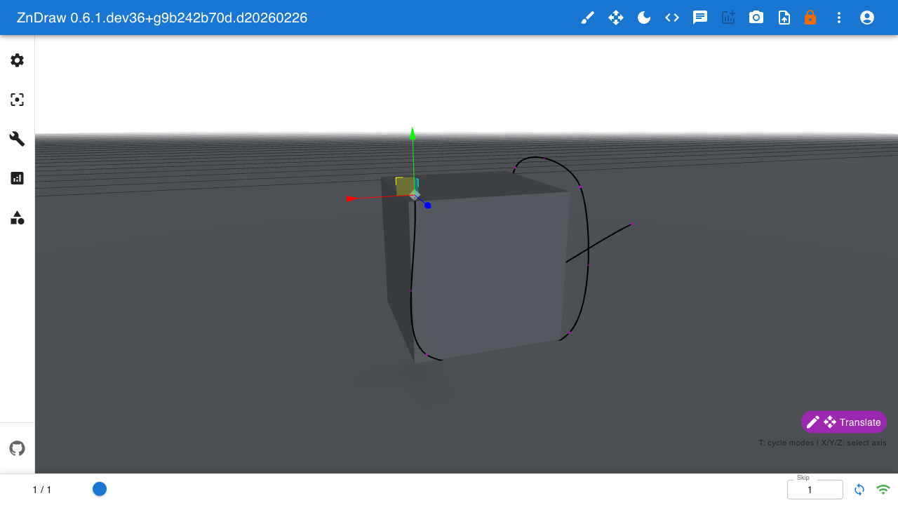
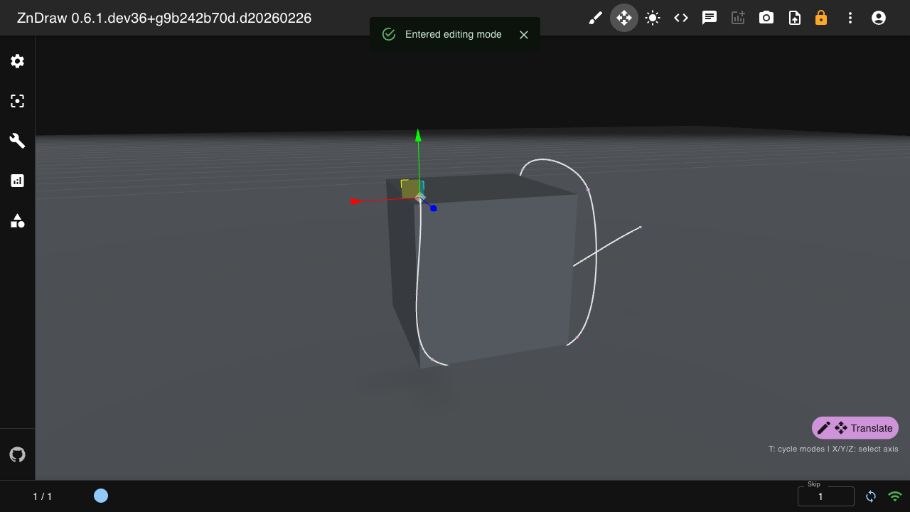
Editing Mode

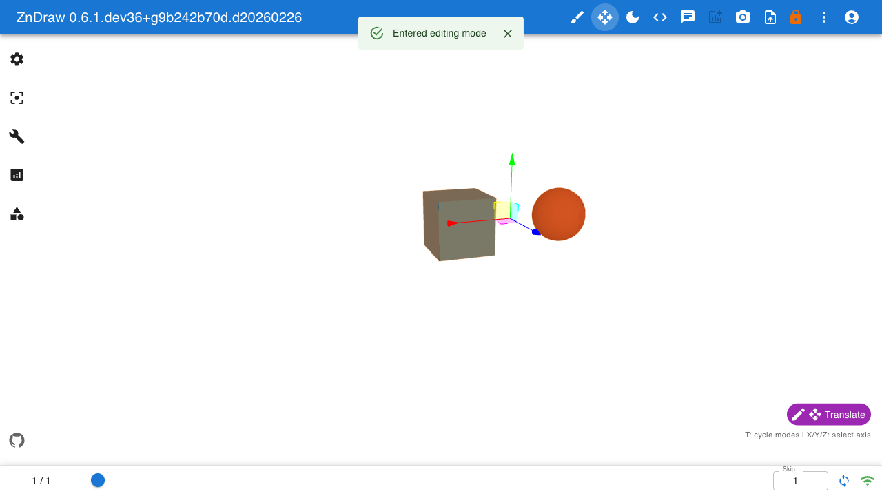
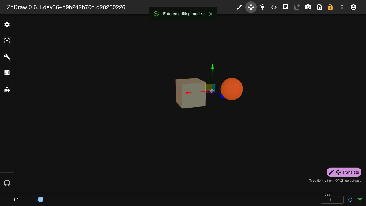
Transform geometries interactively using translate, rotate, and scale controls.

Entering Editing Mode:

1. Press E to enter editing mode (from view mode)

2. Select geometry instances by clicking on them

3. Use the transform gizmo to manipulate selected objects

4. Press T to cycle between translate, rotate, and scale modes

5. Hold X, Y, or Z to constrain movement to a single axis

6. Press S to save changes

7. Press E again to exit and return to view mode

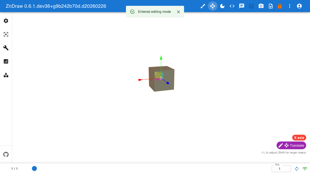
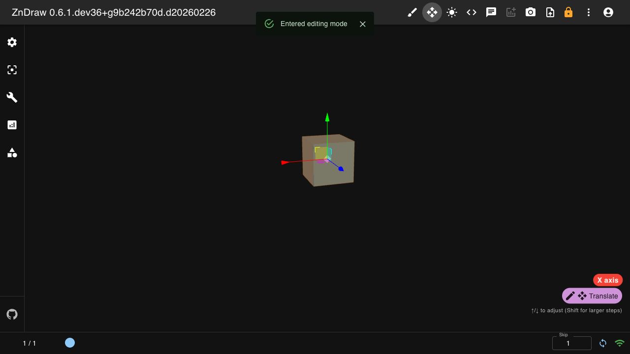
When holding an axis key, a colored chip indicates the active constraint.

Editing Curves:

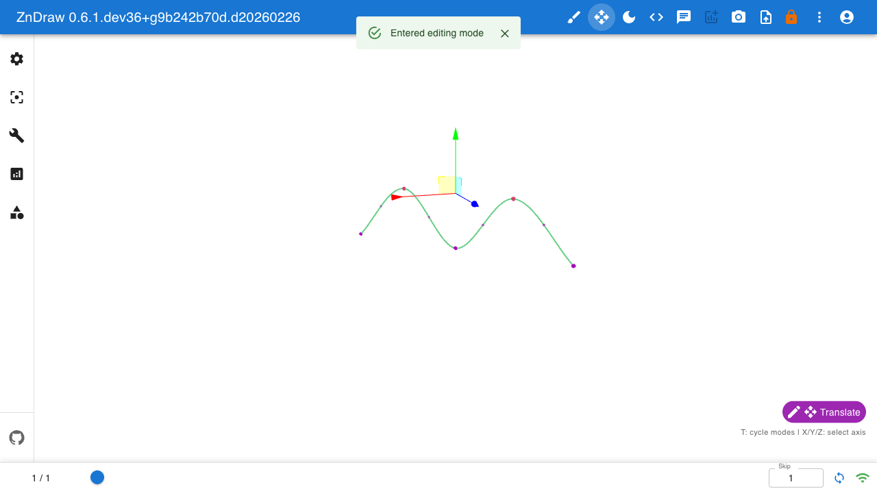
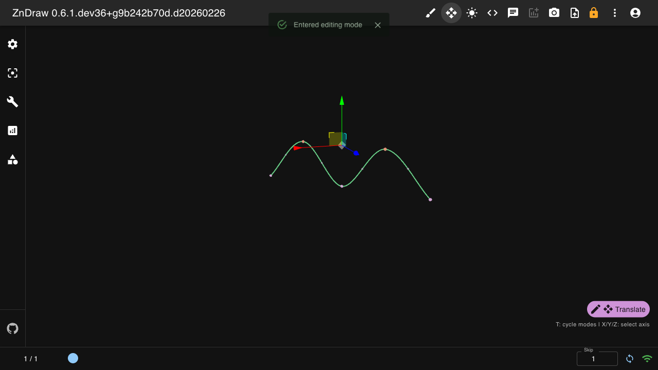
In editing mode, curves display virtual markers between control points. Click a virtual marker to insert a new control point at that position. Use Delete or Backspace to remove selected markers.

Note

See Keyboard Shortcuts for all controls.

Dynamic Properties

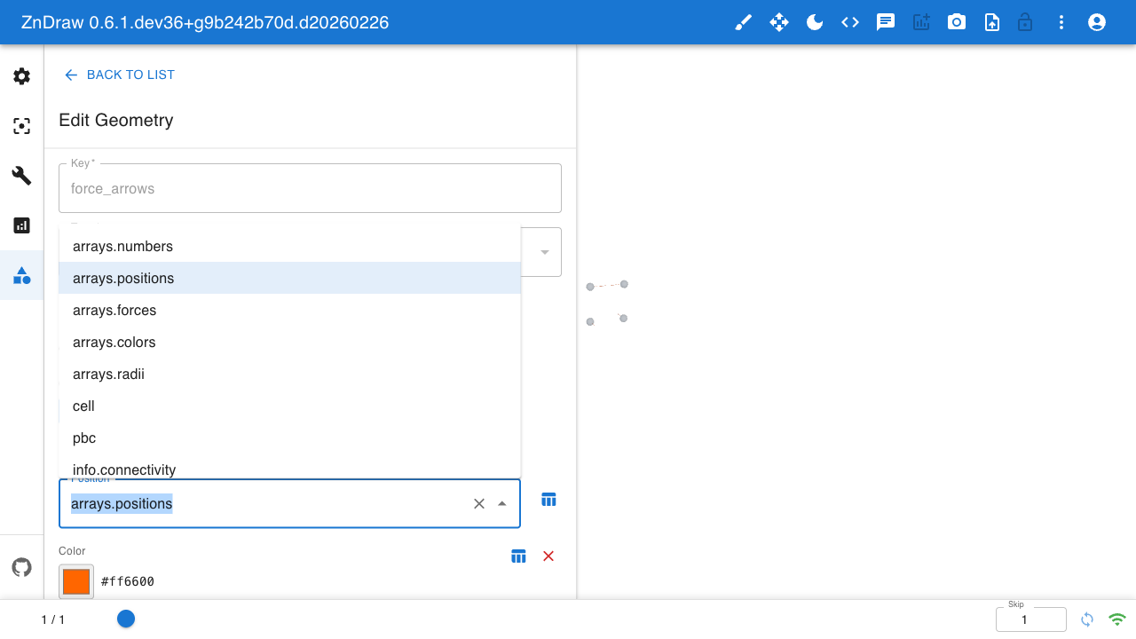
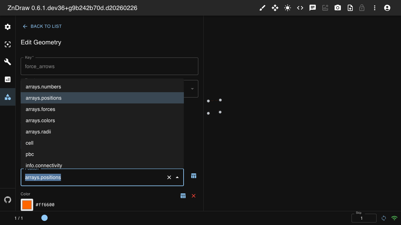
Geometry properties like position and direction can reference atom data dynamically. Instead of specifying fixed coordinates, use string references to atom arrays:

import numpy as np
from zndraw.geometries import Arrow

# Create atoms with calculated forces
atoms = ase.Atoms("H4", positions=[(0, 0, 0), (2, 0, 0), (0, 2, 0), (2, 2, 0)])
atoms.arrays["forces"] = np.array([
    [0, 0, 1], [0, 0, -1], [1, 0, 0], [-1, 0, 0]
], dtype=float)
vis.append(atoms)

# Create arrows showing forces at each atom position
vis.geometries["force_arrows"] = Arrow(
    position="arrays.positions",  # Reference atom positions
    direction="arrays.forces",     # Reference force vectors
    color=["#ff6600"],
    radius=0.1,
)

Available dynamic property references are computed from the atoms.info, atoms.arrays, and if available, atoms.calc.results dictionaries:

• arrays.positions - Atom positions

• arrays.numbers - Atomic numbers

• arrays.colors - Per-atom colors

• arrays.radii - Per-atom radii

• arrays.forces - Calculated forces (if available)

• calc.energy - Calculated energy

• info.connectivity - Bond connectivity

Constraint Visualization

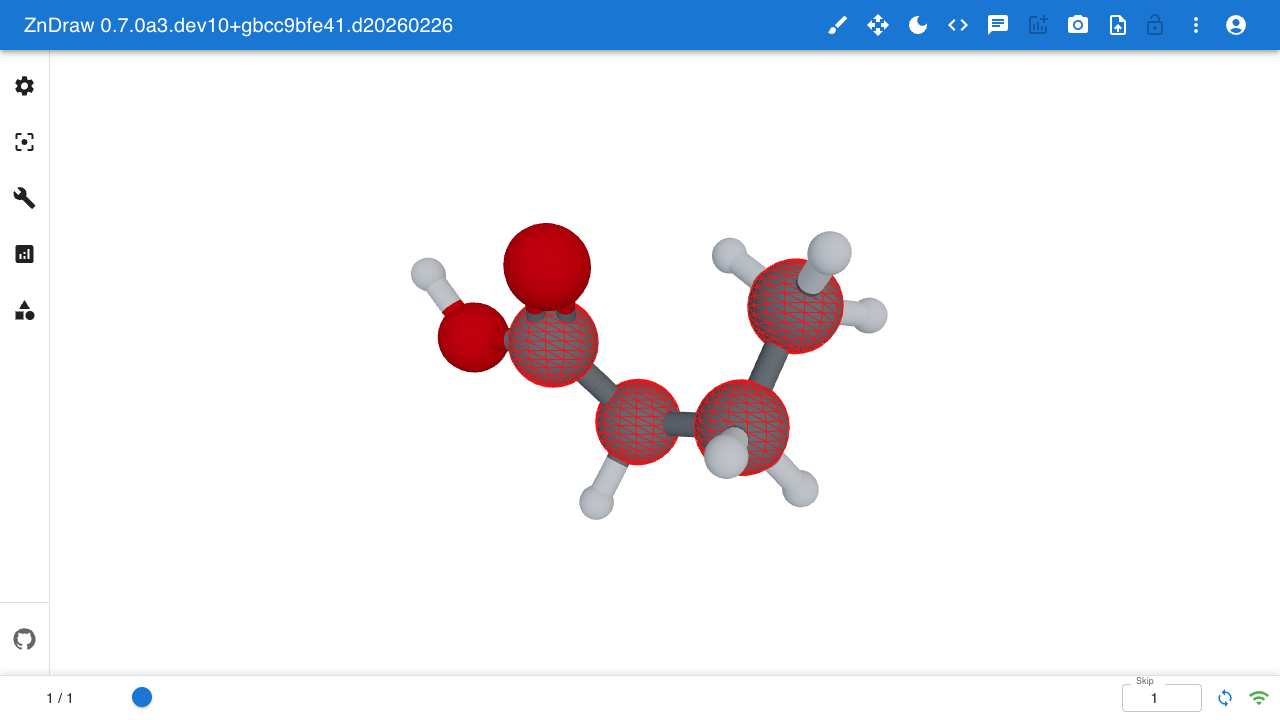
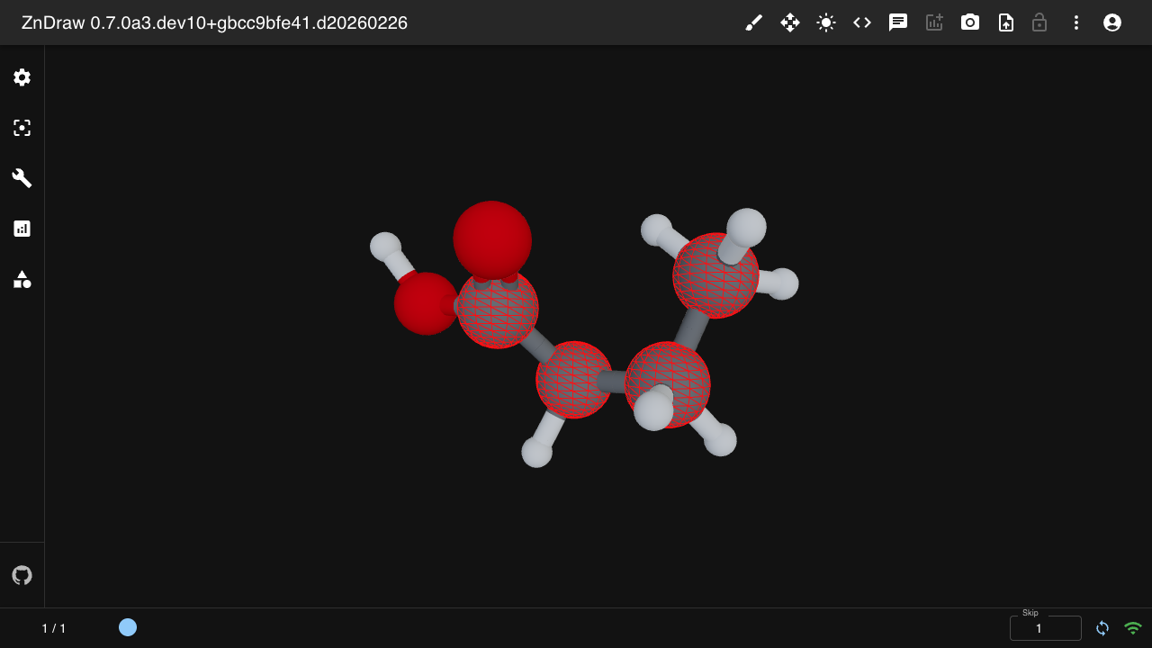
ZnDraw automatically visualizes atomic constraints. When you upload atoms with ASE constraints, a constraints-fixed-atoms geometry overlays red wireframe spheres on the constrained atoms.

from molify import smiles2conformers
from ase.constraints import FixAtoms
from zndraw import ZnDraw

# Create butyric acid and constrain the carbon chain
atoms = smiles2conformers("CCCC(=O)O", numConfs=1)[0]
carbon_indices = [i for i, s in enumerate(atoms.symbols) if s == "C"]
atoms.set_constraint(FixAtoms(indices=carbon_indices))

vis = ZnDraw(url="http://localhost:8000")
vis.append(atoms)

The constrained carbon atoms will appear with a red wireframe sphere overlay, while the remaining atoms are undecorated.

Customization: Open the geometry panel and click constraints-fixed-atoms to change the color, scale, or target a different constraint. The Transform Editor shows a dropdown of all constraints in the current frame — select one to switch which atoms are highlighted.

Isosurface

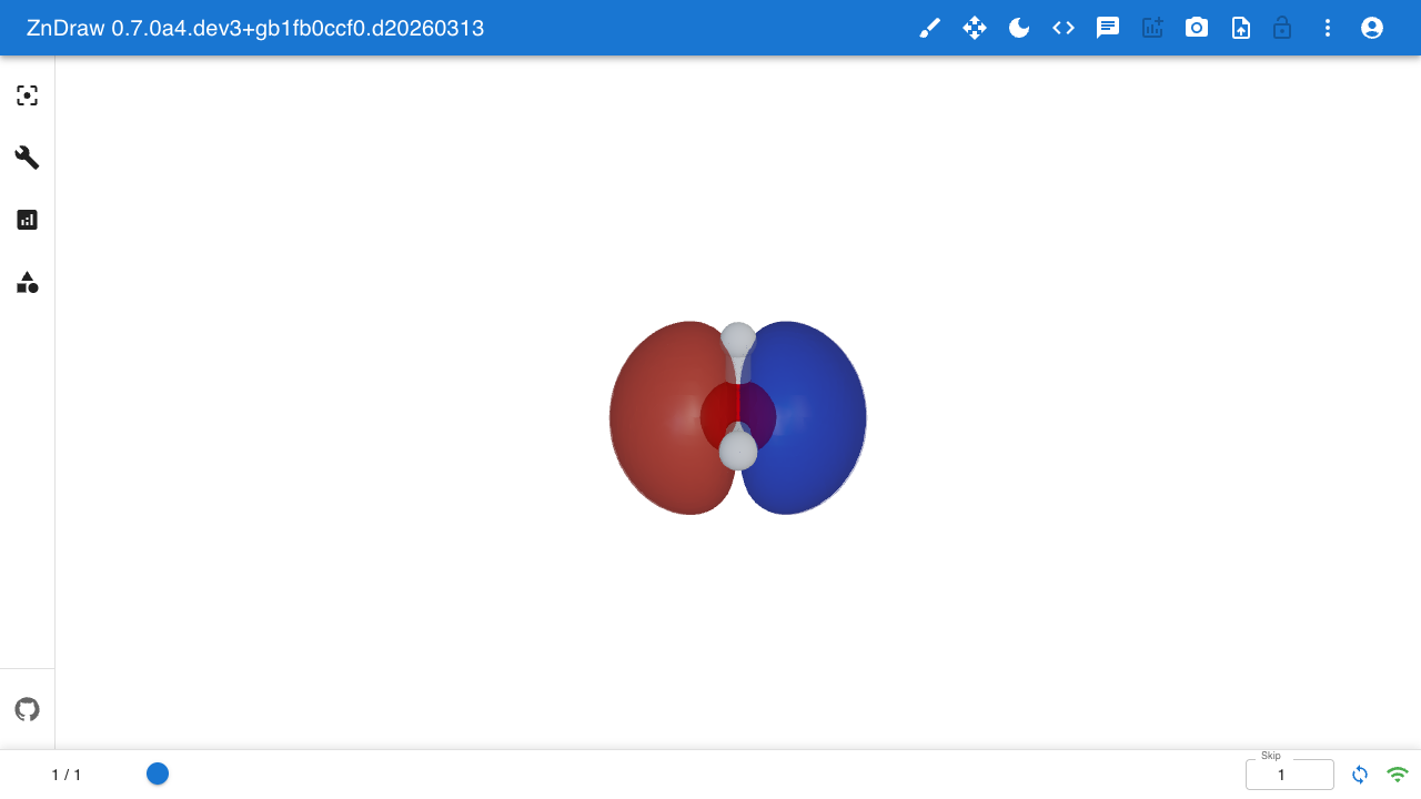
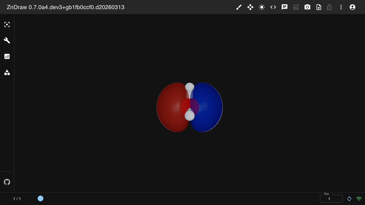
Visualize volumetric data (e.g. molecular orbitals, electron densities) as 3D isosurfaces. The cube_key points to a frame info key containing a dict with:

• grid: 3D float array of shape (Nx, Ny, Nz) — scalar field values

• origin: 3-vector — world-space origin of the grid (Angstrom)

• cell: (3, 3) matrix — axis vectors spanning the grid (Angstrom)

import numpy as np
from zndraw.geometries import Isosurface

# Store volumetric data in a frame
atoms.info["orbital_homo"] = {
    "grid": orbital_data,     # np.ndarray (Nx, Ny, Nz)
    "origin": origin,         # np.ndarray (3,)
    "cell": cell_vectors,     # np.ndarray (3, 3)
}
vis.append(atoms)

# Create positive and negative lobes
vis.geometries["homo_pos"] = Isosurface(
    cube_key="info.orbital_homo", isovalue=0.02, color="#2244CC",
)
vis.geometries["homo_neg"] = Isosurface(
    cube_key="info.orbital_homo", isovalue=-0.02, color="#CC4422",
)

Parameters:

• cube_key: Frame info key for the volumetric data dict (dynamic dropdown in UI)

• isovalue: Scalar threshold for surface extraction (default 0.02, range -0.25 to 0.25)

• resolution: Mesh resolution, 0 = coarse/fast, 1 = fine/slow (default 1.0)

• opacity: Surface transparency, 0 = invisible, 1 = opaque (default 0.6)

• color: Surface color as hex string (default #2244CC)

Analysis & Figures

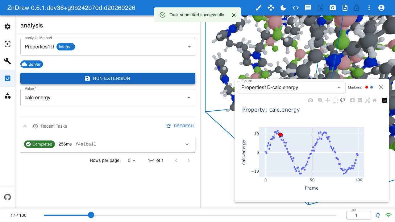
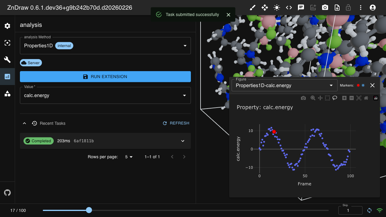
Display interactive Plotly figures with vis.figures:

import plotly.express as px
import pandas as pd

# Create figure from data
df = pd.DataFrame({
    "frame": range(len(vis)),
    "energy": [atoms.get_potential_energy() for atoms in vis]
})

fig = px.line(df, x="frame", y="energy", title="Energy vs Frame")

# Display in ZnDraw
vis.figures["energy_plot"] = fig

# Remove figure
del vis.figures["energy_plot"]

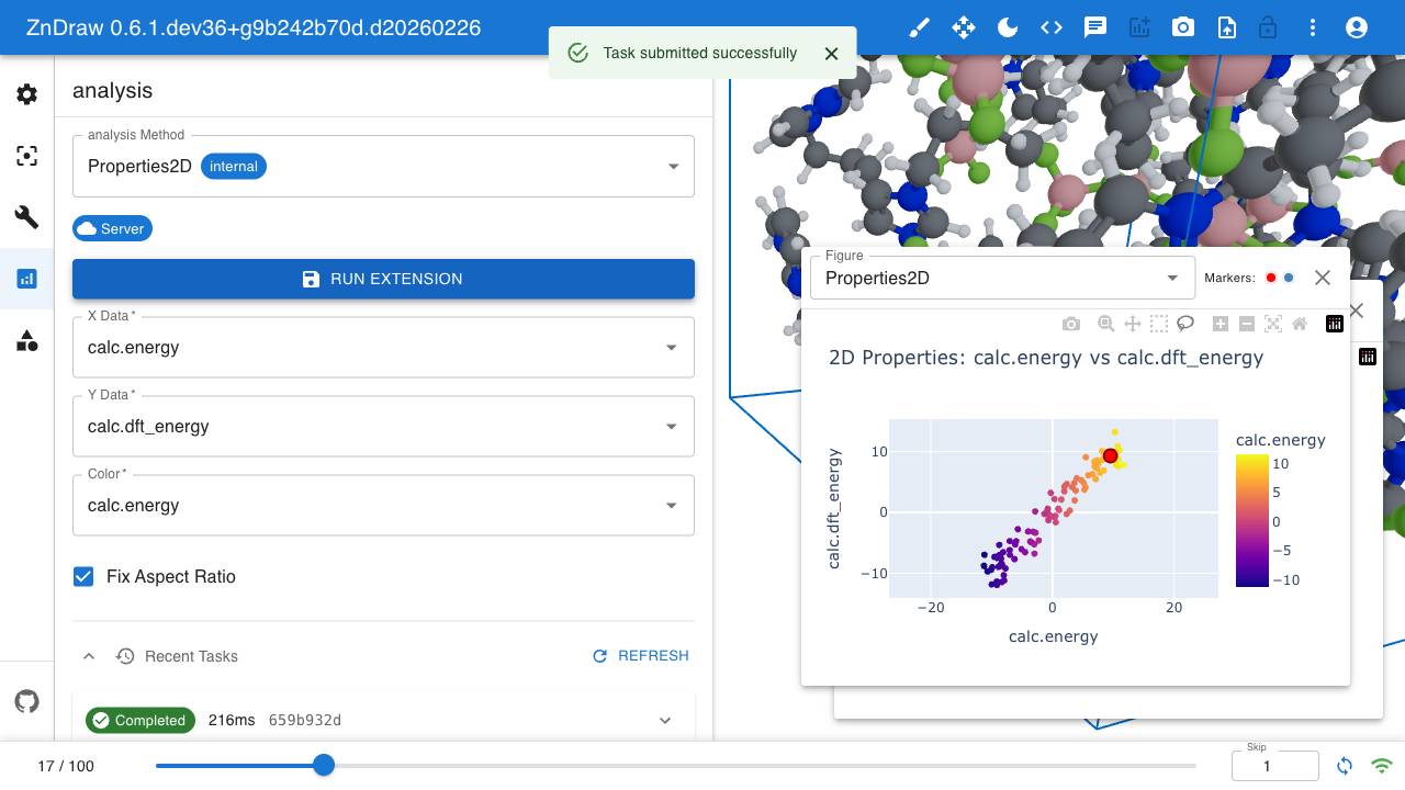
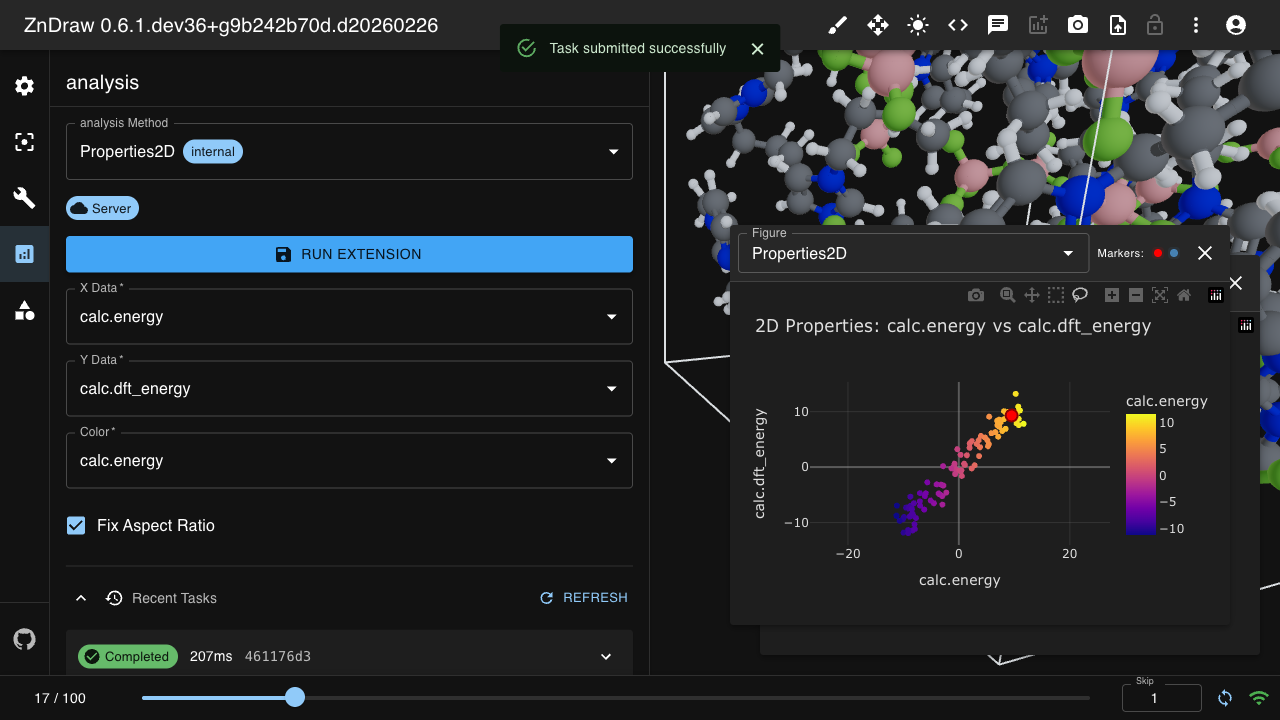
2D analysis with scatter plots:

# 2D scatter plot
df = pd.DataFrame({
    "ml_energy": [...],
    "dft_energy": [...]
})

fig = px.scatter(df, x="ml_energy", y="dft_energy", title="ML vs DFT Energy")

vis.figures["comparison"] = fig

Molecule Building

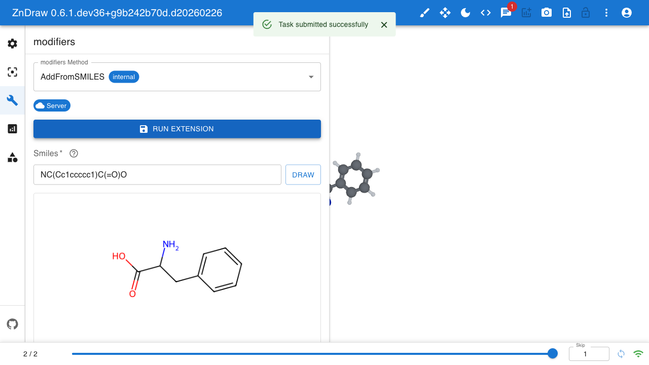
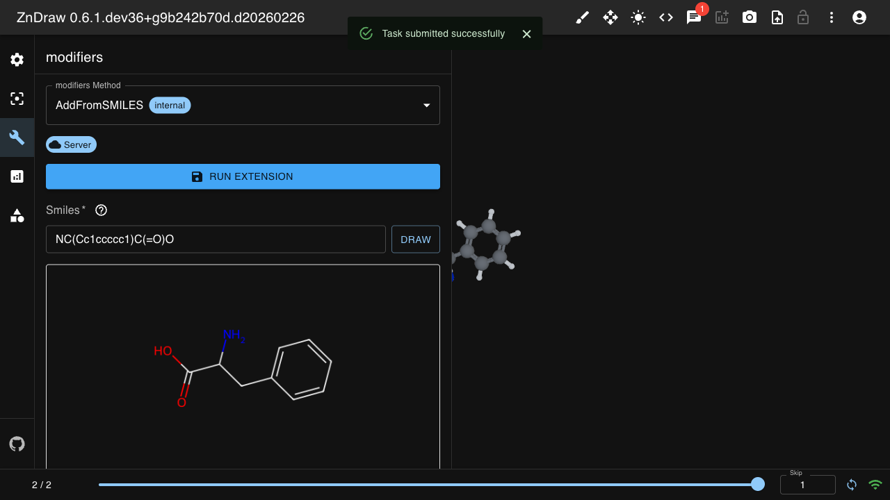
Build molecules from SMILES strings using the molecule builder:

• Add molecules from SMILES notation

• Use the Ketcher molecular editor

• Pack molecules into simulation boxes

Ketcher Editor:

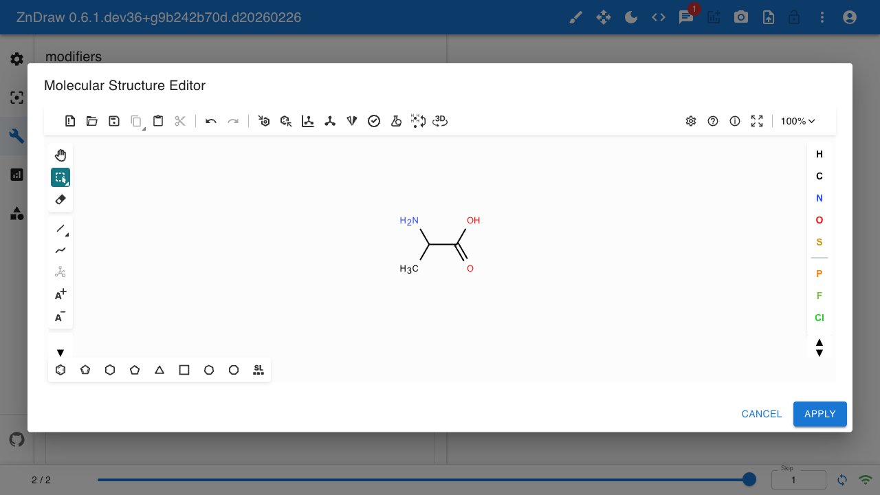
Note

The Ketcher editor currently does not support dark mode. See Ketcher issue #5353 for more information.

Chat & Logging

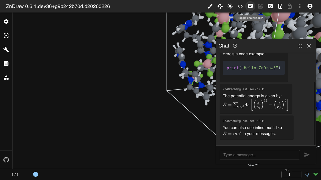
Send messages to the chat panel:

# Send a message
vis.log("Analysis complete!")

# Messages support Markdown and LaTeX
vis.log("Energy: $E = mc^2$")

# Get chat history
messages = vis.get_messages(limit=10)

Frame References

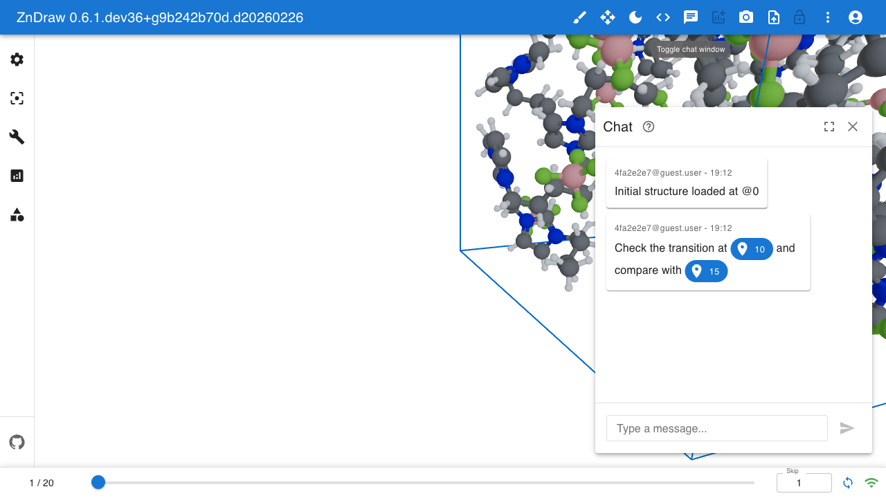
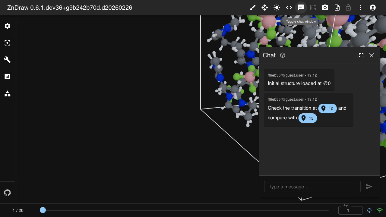
Reference frames in chat messages using @{frame} syntax. Frame references become clickable chips that navigate to the referenced frame:

# Reference specific frames in messages
vis.log("Initial structure at @0")
vis.log("Compare @10 with @15 to see the transition")

Clicking a frame reference chip navigates directly to that frame.

Markdown & Code Blocks

Chat messages support full Markdown rendering including:

• Text formatting: **bold**, *italic*, ~~strikethrough~~

• Lists: Ordered and unordered lists

• Links: [text](url)

• LaTeX math: Inline $E = mc^2$ or block $$\sum_{i=1}^n x_i$$

• Code blocks: Syntax-highlighted code with language specification

vis.log("""
## Results Summary

The simulation converged after **1000 steps**.

Energy: $E = -42.5$ eV

```python
for atom in atoms:
    print(atom.symbol)
```
""")

Progress Bars

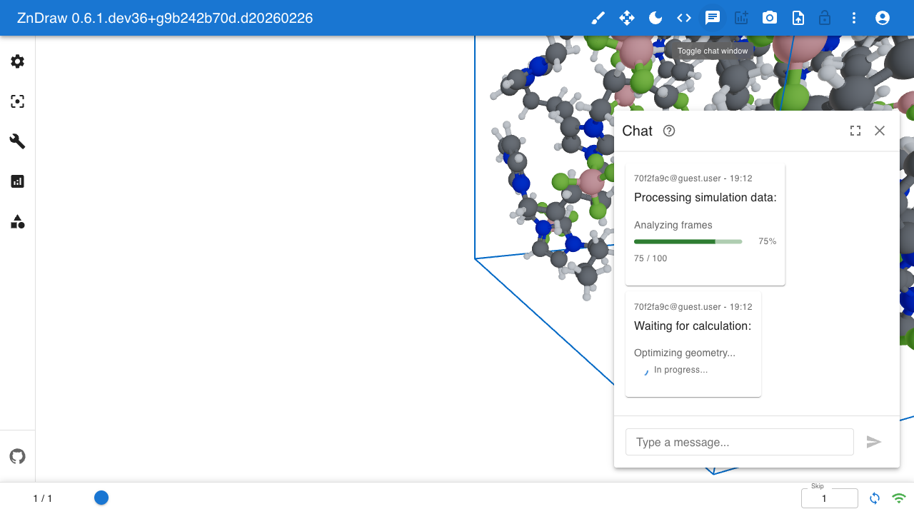
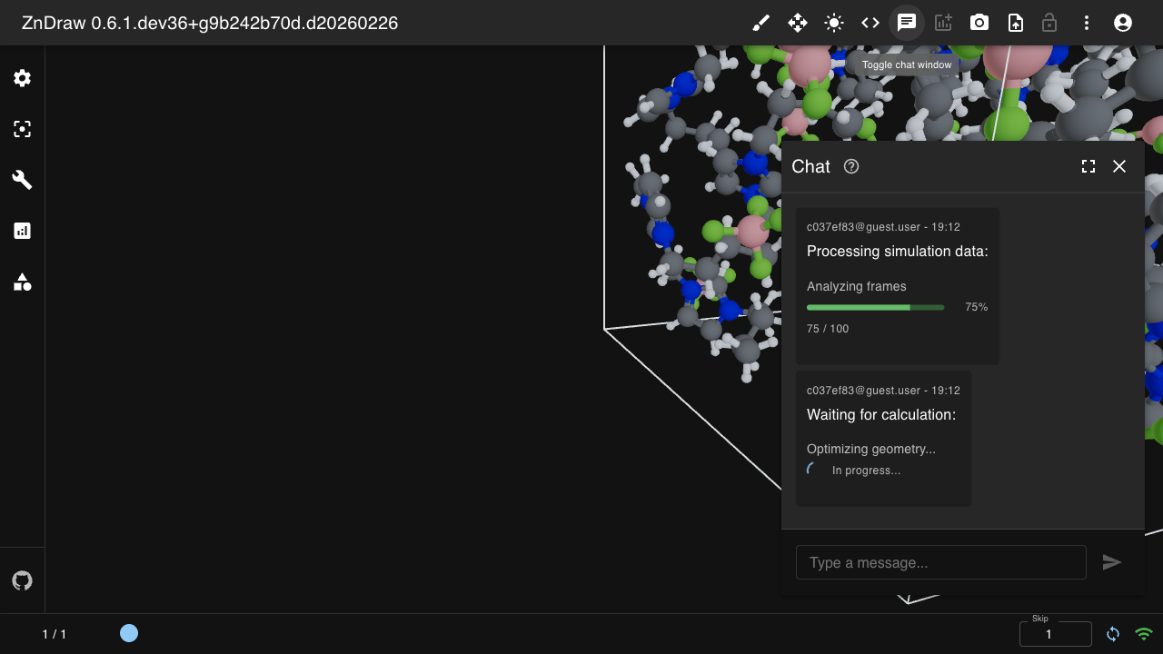
Display progress bars in chat using the progress code block syntax:

vis.log("""
```progress
description: Processing frames
value: 75
max: 100
color: success
```
""")

Parameters:

• value: Current progress value. If omitted, shows an indeterminate spinner.

• min: Minimum value (default: 0)

• max: Maximum value (default: 100)

• description: Label text displayed above the progress bar

• color: MUI color - primary, secondary, success, error, warning, info (default: primary)

The progress bar displays the percentage and the current value relative to max. For long-running operations, consider using ZnDrawTqdm instead, which provides real-time updates.

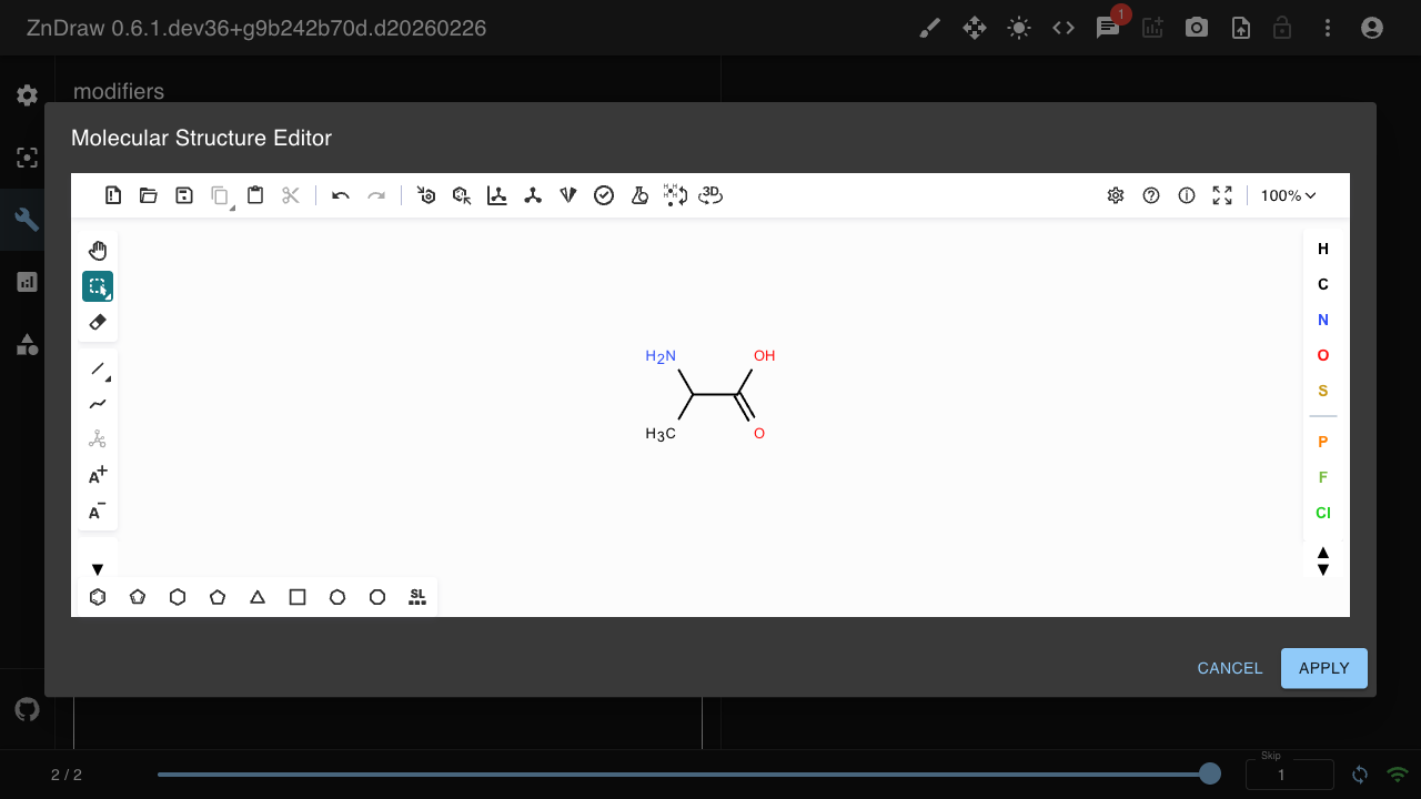
Molecule Structures

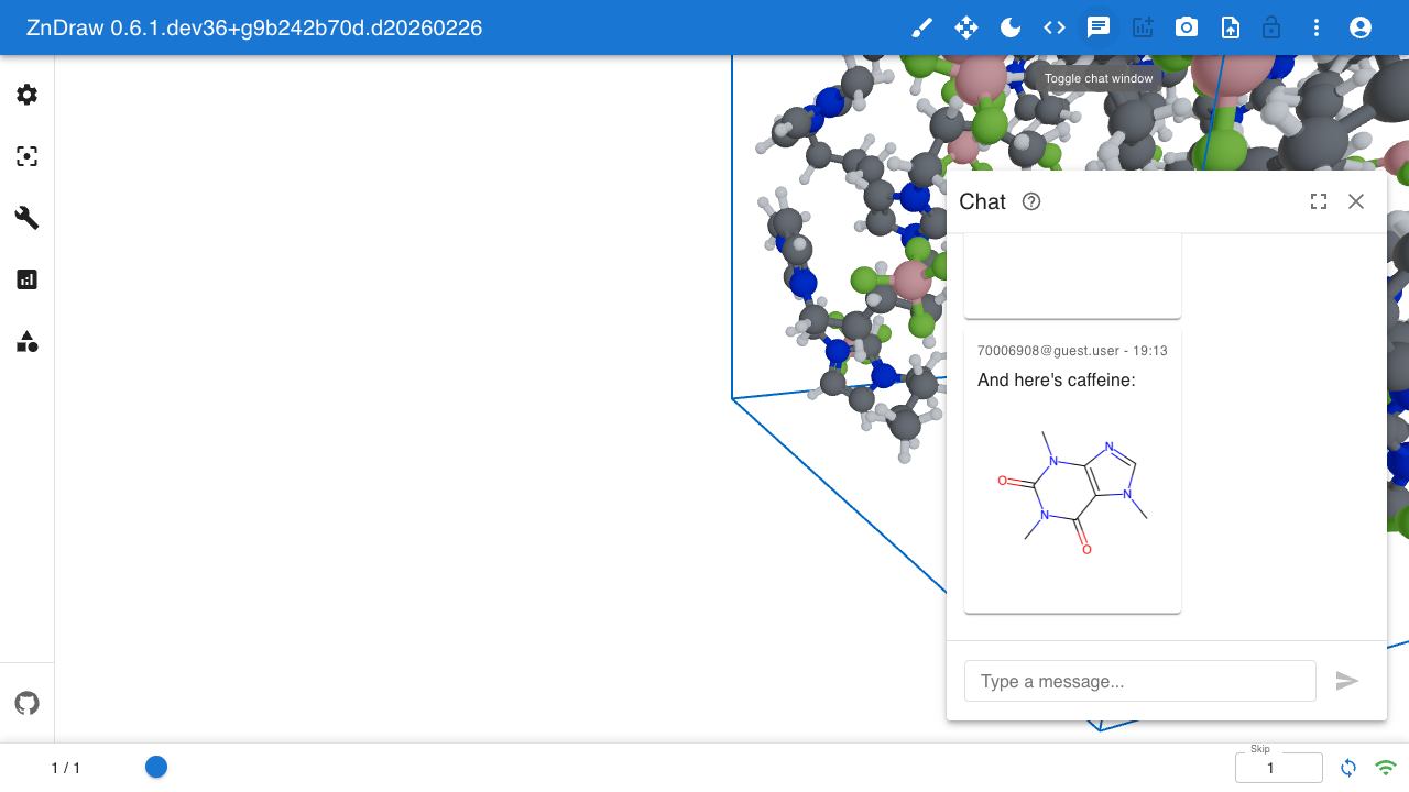
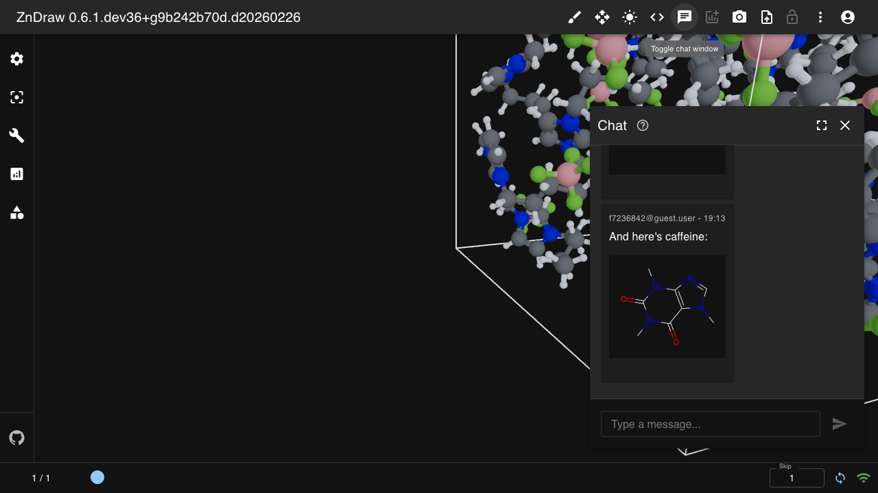
Display molecule structures in chat using SMILES notation with the smiles code block syntax:

vis.log("""
```smiles
CCO
```
""")

The SMILES string is rendered as a 2D molecule structure image using RDKit.

Property Inspector

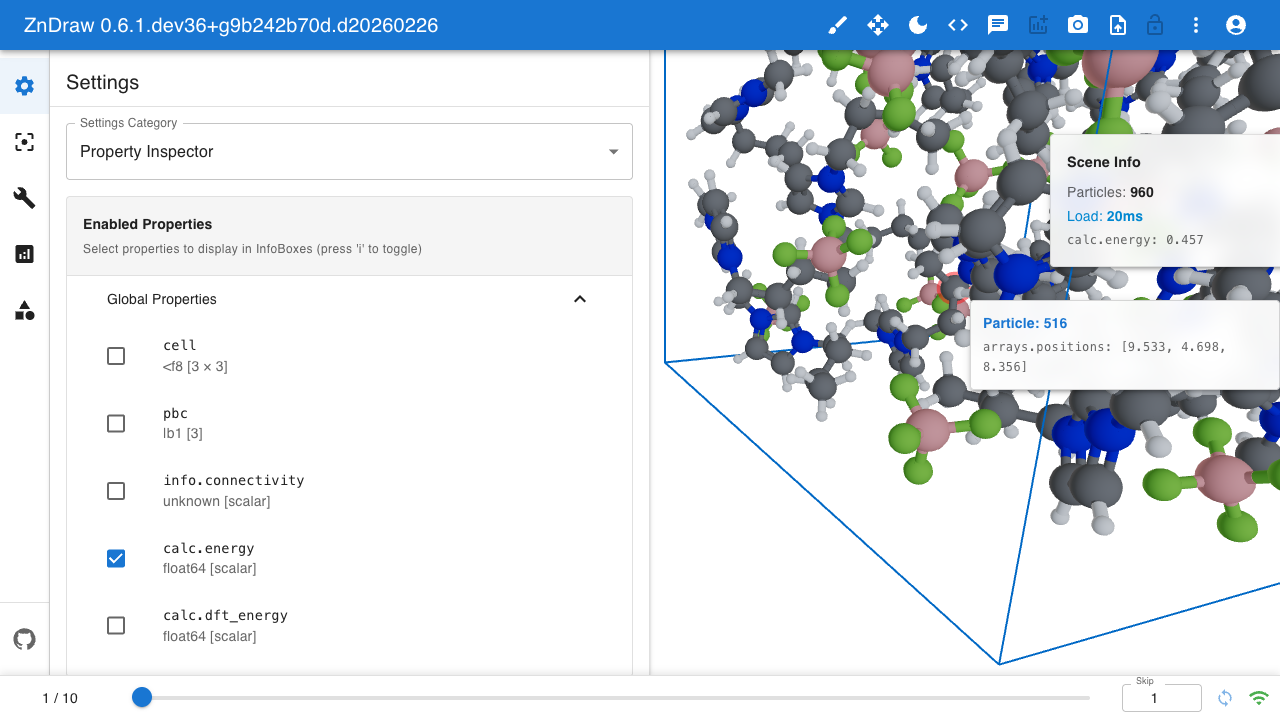
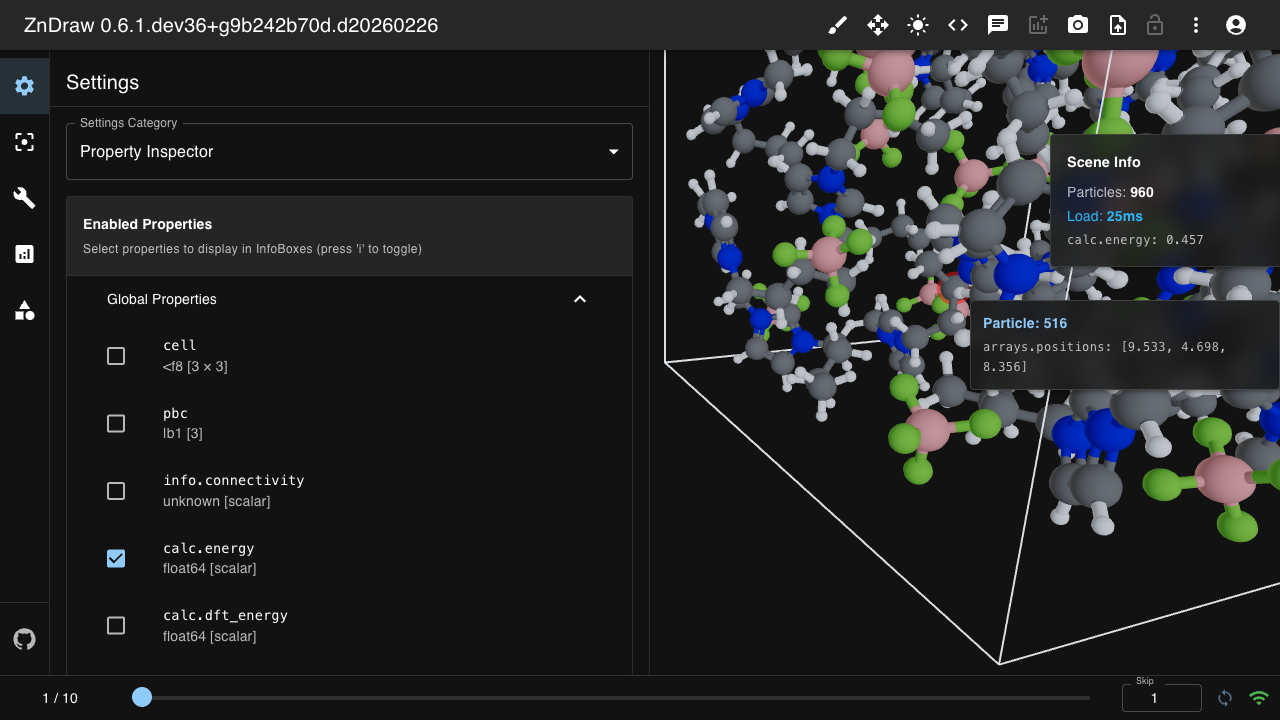
The property inspector displays frame properties in floating info boxes. Press i to toggle visibility. Configure which properties to display via settings:

# Enable properties in the inspector
vis.sessions["<sessionId>"].settings.property_inspector.enabled_properties = [
    "calc.energy",
    "calc.forces",
]

Two info boxes are available:

• Scene Info (top-right): Displays global properties like calc.energy

• Hover Info (follows cursor): Shows per-particle properties when hovering over atoms

Properties are automatically categorized based on their shape:

• Global: Scalar values or arrays not matching particle count

• Per-particle: Arrays with first dimension equal to particle count

Browser Sessions

Access connected browser windows via vis.sessions. Each frontend session has its own camera and rendering settings:

# List all connected browser sessions
for session_id in vis.sessions:
    print(session_id)

# Access a specific session
session = vis.sessions["abc-123"]

# Get/set camera for that browser window
cam = session.camera
print(cam.position, cam.target)

# Update camera position
from zndraw.geometries import Camera
session.camera = Camera(position=(10, 5, 10), target=(0, 0, 0), fov=60)

# Access session settings
settings = session.settings
settings.studio_lighting.key_light = 1.5  # adjust settings

Note

Only frontend browser windows appear in vis.sessions. Python API clients do not create entries here.

Progress Tracking

Track long-running operations with ZnDrawTqdm:

from zndraw import ZnDrawTqdm

for item in ZnDrawTqdm(items, vis=vis, description="Processing data"):
    process(item)

The progress bar appears in the UI with the current message and completion percentage.

Lock Mechanism

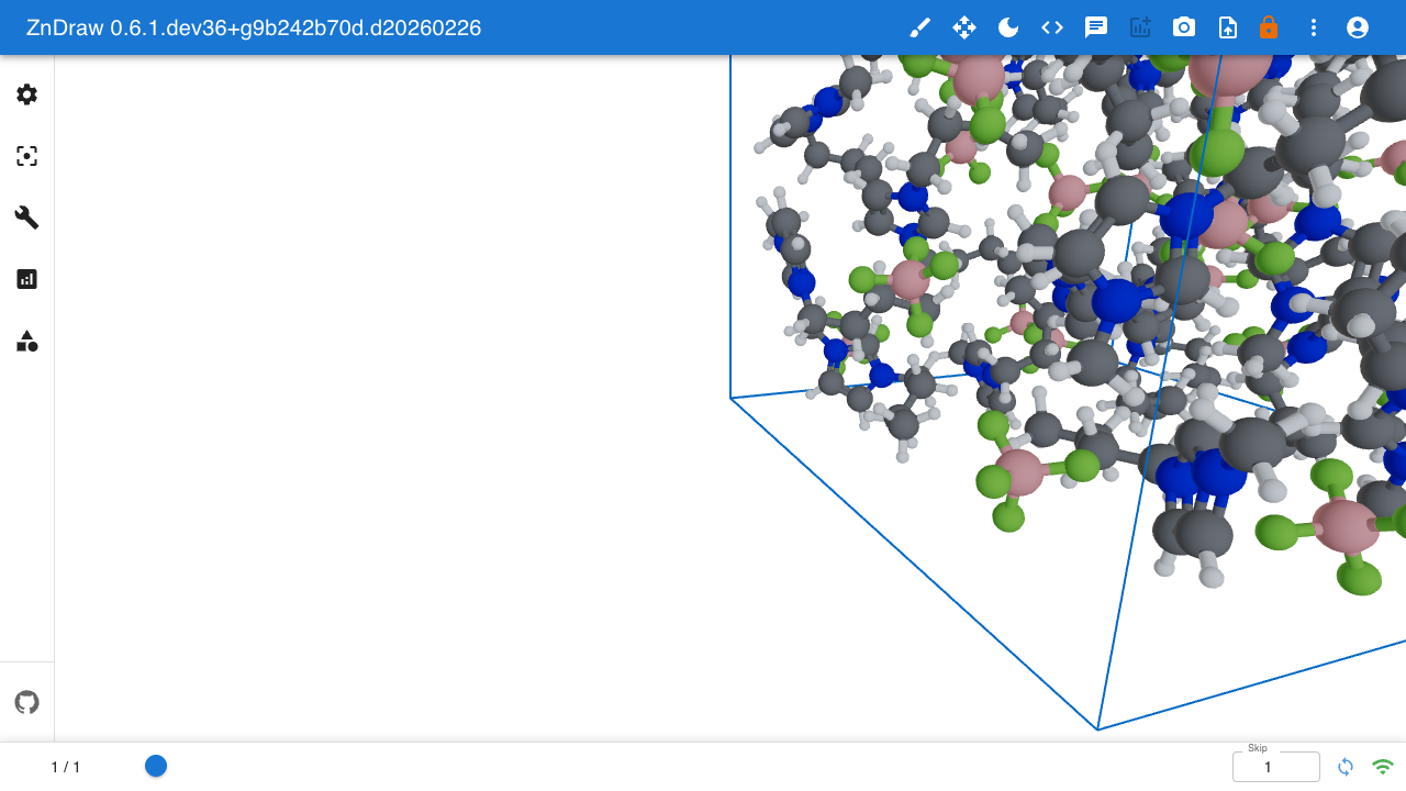
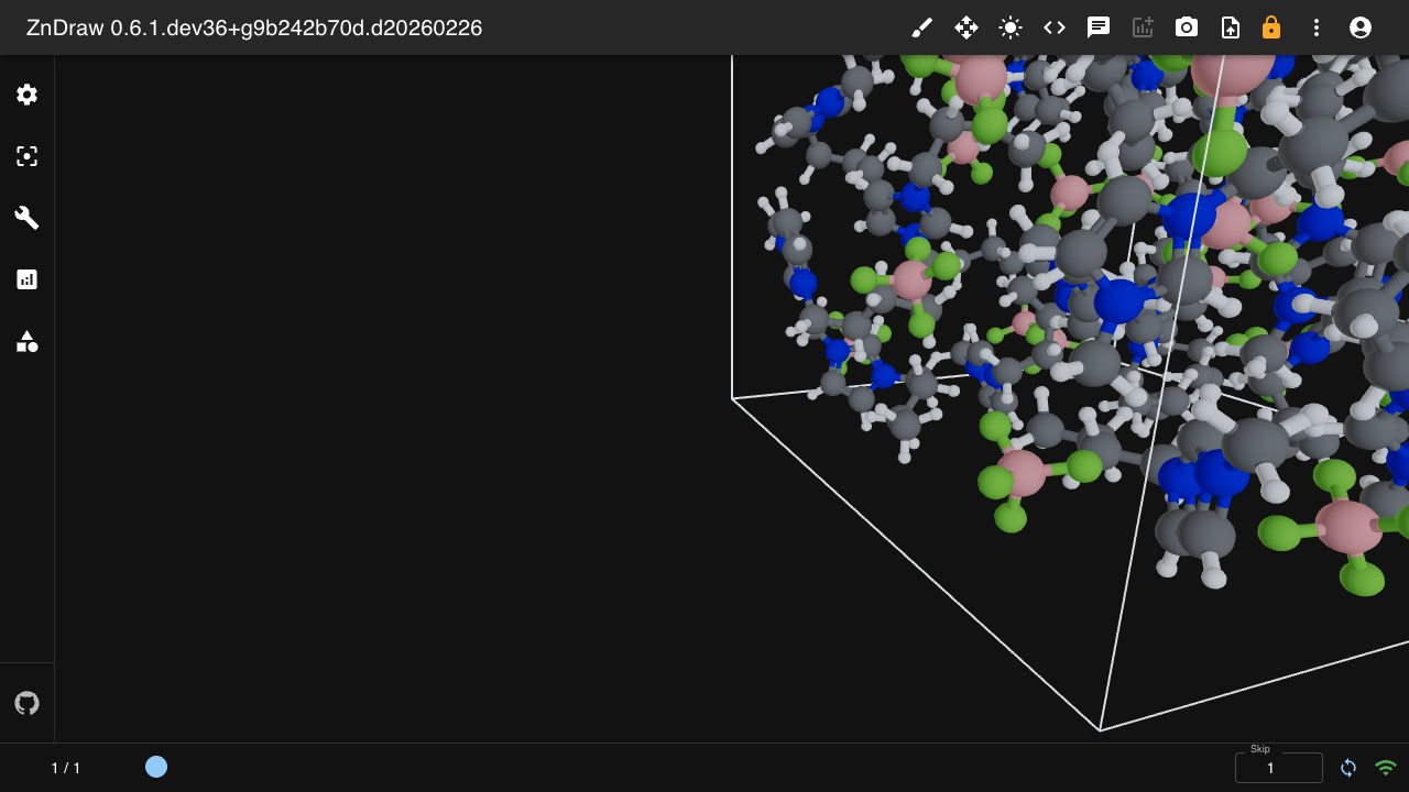
Use vis.get_lock() for safe batch operations that prevent concurrent modifications:

# Lock the room during bulk operations
with vis.get_lock(msg="Uploading trajectory..."):
    for atoms in trajectory:
        vis.append(atoms)

# Lock specific targets for fine-grained control
with vis.get_lock(target="step"):
    vis.step = 42

While a lock is held, other clients see a locked indicator (shown above) and cannot modify the locked resources. The lock message is displayed in the UI so users know what operation is in progress. This is useful when uploading large trajectories or performing multi-step operations that should not be interrupted.

Custom Extensions

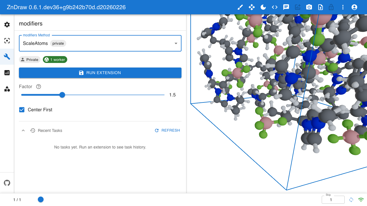
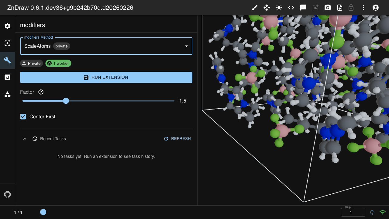
ZnDraw supports custom extensions for modifiers, selections, and analysis. Subclass Extension, set a category, and implement run():

from pydantic import Field
from zndraw import ZnDraw, Extension, Category

class ScaleAtoms(Extension):
    """Scale atom positions by a factor."""

    category = Category.MODIFIER  # or SELECTION or ANALYSIS
    factor: float = Field(
        1.5, ge=0.1, le=5.0,
        description="Scale factor",
        json_schema_extra={"format": "range"},
    )
    center_first: bool = Field(
        True,
        description="Center atoms before scaling",
    )

    def run(self, vis, **kwargs):
        atoms = vis.atoms.copy()
        if self.center_first:
            atoms.positions -= atoms.get_center_of_mass()
        atoms.positions *= self.factor
        vis.append(atoms)
        vis.step = len(vis) - 1

Extension Categories

Extensions are categorized by their purpose:

• Category.MODIFIER: Modify atomic structures (e.g., delete, rotate, translate)

• Category.SELECTION: Select atoms (e.g., by type, neighbors, random)

• Category.ANALYSIS: Analyze data and create plots (e.g., properties, correlations)

Registering Extensions

Use register_job() to make an extension available in the UI.

Room-scoped (default):

vis = ZnDraw()
vis.register_job(ScaleAtoms)  # visible only in vis.room
vis.wait()

Global (admin-only):

Global extensions are visible in all rooms. Only admin users can register them — non-admin users receive a PermissionError (HTTP 403).

from zndraw import GLOBAL_ROOM

vis = ZnDraw(url="http://localhost:4567", user="admin@example.com", password="...")
vis.register_job(ScaleAtoms, room=GLOBAL_ROOM)  # visible in all rooms
vis.wait()

Note

The @global and @internal sigils are still supported for system-scoped jobs. They are not composed addresses — they are reserved system rooms.

Explicit room:

vis.register_job(ScaleAtoms, room="123e4567-e89b-12d3-a456-426614174000/my-room")

Passing Runtime State (run_kwargs)

Heavy objects that should live in worker memory (e.g. ML models, database connections) can be passed at registration time via run_kwargs. These kwargs are forwarded to extension.run() on every task execution without being serialized:

import torch

model = torch.load("model.pt")

class Predict(Extension):
    category = Category.MODIFIER
    temperature: float = 1.0

    def run(self, vis, *, model=None, **kwargs):
        atoms = vis[vis.step]
        result = model(atoms, self.temperature)
        vis.append(result)
        vis.step = len(vis) - 1

vis = ZnDraw()
vis.register_job(Predict, run_kwargs={"model": model})
vis.wait()

The run_kwargs dict is stored in the worker process and never sent to the server. This means values can be non-serializable (torch models, open file handles, etc.). Each invocation of run() receives the same object references.

Extension Scopes

Every extension is prefixed by its scope:

The full name of an extension follows the pattern <scope>:<category>:<name>, e.g. @global:modifiers:ScaleAtoms.

Running Extensions

Submit an extension for execution via vis.run(). This returns a TaskHandle that can be polled or awaited:

# Run a built-in extension
task = vis.run("@internal:modifiers:Delete")
task.wait(timeout=30)

# Run with parameters
task = vis.run("@global:modifiers:ScaleAtoms", factor=2.0, center_first=True)
task.wait()

# Check status
print(task.status)  # "completed" or "failed"

Discover available extensions with vis.extensions:

# List all extension names
list(vis.extensions)

# Get schema for a specific extension
vis.extensions["@internal:modifiers:Delete"]

Worker Lifecycle

When you call register_job(), the client connects via Socket.IO and starts a background worker that claims and executes tasks. Call vis.wait() to block until the process is interrupted:

vis = ZnDraw()
vis.register_job(ExtensionA)
vis.register_job(ExtensionB)
vis.wait()  # blocks until Ctrl+C

The worker sends heartbeats to the server. On disconnect, all registered jobs are cleaned up automatically.

Providers

Providers are read-only data source handlers that let extensions access external resources (filesystems, databases, etc.) through the worker process.

Filesystem provider (convenience)

register_fs() registers an fsspec filesystem and the built-in LoadFile extension in one call:

import fsspec

vis = ZnDraw()
vis.register_fs(fsspec.filesystem("file"), name="local")
vis.wait()

Users can then load files from the UI via the LoadFile modifier.

Custom providers

Subclass Provider, implement read(handler), and register with register_provider():

from zndraw_joblib import Provider

class DBLookup(Provider):
    category = "database"
    query: str = ""

    def read(self, handler):
        # handler is whatever you pass to register_provider()
        return handler.execute(self.query).fetchall()

vis.register_provider(DBLookup, name="my-db", handler=db_connection)

Extensions access providers via the providers kwarg passed to run():

class MyExtension(Extension):
    category = Category.MODIFIER

    def run(self, vis, **kwargs):
        providers = kwargs.get("providers") or {}
        db = providers.get(f"{vis.room}:database:my-db")
        rows = db.execute("SELECT ...").fetchall()
        ...

Provider names follow the pattern {room}:{category}:{name}.

Schema Customization

Use json_schema_extra and Field options to customize how fields appear in the UI:

Slider Input

factor: float = Field(
    1.0, ge=0.0, le=10.0,
    json_schema_extra={"format": "range"},
)

Dynamic Dropdowns

Populate dropdowns at runtime from available data:

# Dropdown from geometry names (filtered to Curves)
curve: str = Field(
    "curve",
    json_schema_extra={
        "x-custom-type": "dynamic-enum",
        "x-features": ["dynamic-geometries"],
        "x-geometry-filter": "Curve",
    },
)

# Dropdown from atom/frame properties
property: str = Field(
    ...,
    json_schema_extra={
        "x-custom-type": "dynamic-enum",
        "x-features": ["dynamic-atom-props"],
    },
)

SMILES Input with Ketcher Editor

smiles: str = Field(
    ...,
    json_schema_extra={"x-custom-type": "smiles"},
)

Available Options

Option	Description
"format": "range"	Render as slider (requires ge/le bounds)
"x-custom-type": "smiles"	SMILES input with Ketcher editor button
"x-custom-type": "dynamic-enum"	Runtime-populated dropdown
"x-features": ["dynamic-geometries"]	Populate from geometry names
"x-features": ["dynamic-atom-props"]	Populate from atom/frame properties
"x-geometry-filter": "Curve"	Filter geometries by type

Custom Filesystems

Register any fsspec-compatible filesystem to browse and load files from the UI:

from fsspec.implementations.dirfs import DirFileSystem

vis.register_filesystem(DirFileSystem(path="."), "local")

All fsspec-compatible filesystems are supported, including S3, GCS, Azure, HDFS, and more.